Getting started

This vignette walks through a basic workflow using cd4backcalc: simulate HIV diagnosis data, fit a CD4-staged back-calculation model, assess convergence and goodness of fit, and plot the model estimates.

library(cd4backcalc)
library(patchwork)

Simulate data

We first simulate HIV diagnosis data using simulate_diagnoses(). This function propagates a specified number of HIV infections through the back-calculation model to generate diagnoses over time. Key arguments control the simulation scenario (sim_type), whether to include migration, RITA, and/or age structure, and a seed for reproducibility.

sim_diags <- simulate_diagnoses(sim_type = "combo_3", sim_seed = 123)

If you are working with real data rather than simulated data, you can skip this step and pass a pre-formatted stan_data list directly to run_backcalc().

For real data, the input to run_backcalc() should be a Stan-ready list containing the diagnosis arrays required for the chosen model. At minimum this includes diagnosis counts (HIV, AIDS, and CD4); migration, RITA, and age-dependent models additionally require the corresponding migration, recency, and age-specific arrays. When fitting real data, pass the matching migration, rita, and age flags explicitly to run_backcalc().

hiv_list_real <- run_backcalc(
  real_stan_data,
  migration = TRUE,
  rita = FALSE,
  age = FALSE
)

We can visualise the simulated data using plot_simulations():

plot_simulations(sim_diags, quantity = "incidence")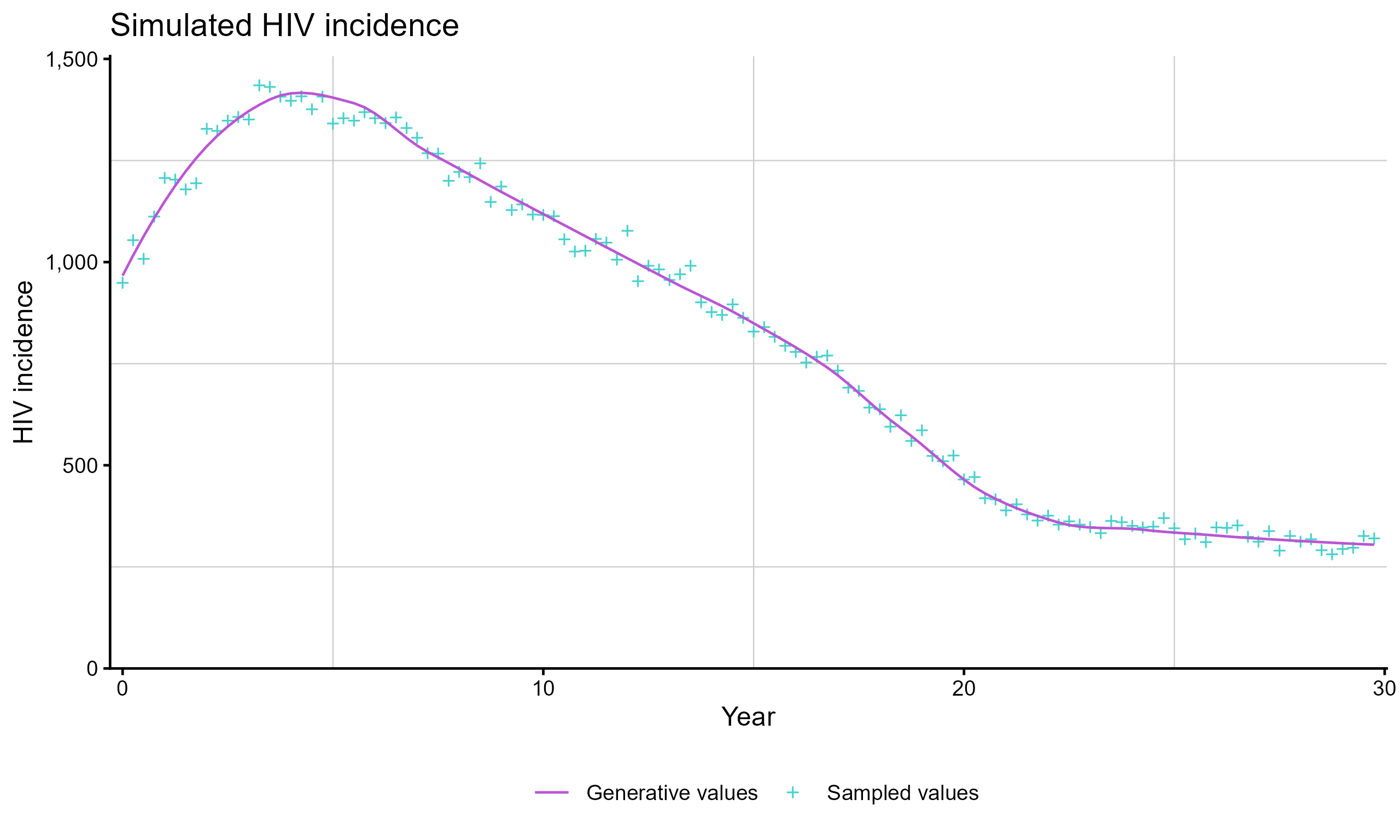

Fit the model

The run_backcalc() function fits the CD4-staged back-calculation model using cmdstanr. By default, each chain runs 1000 warmup and 1000 sampling iterations across 4 chains.

hiv_list <- run_backcalc(sim_diags)

For faster iteration during development, you can reduce the number of iterations and chains:

hiv_list <- run_backcalc(
  sim_diags,
  iter_warmup = 500,
  iter_sampling = 500,
  chains = 2
)

Assess convergence

Use plot_diagnostics() to inspect traceplots and posterior density plots for key parameters:

plot_diagnostics(hiv_list, ntraces = 4)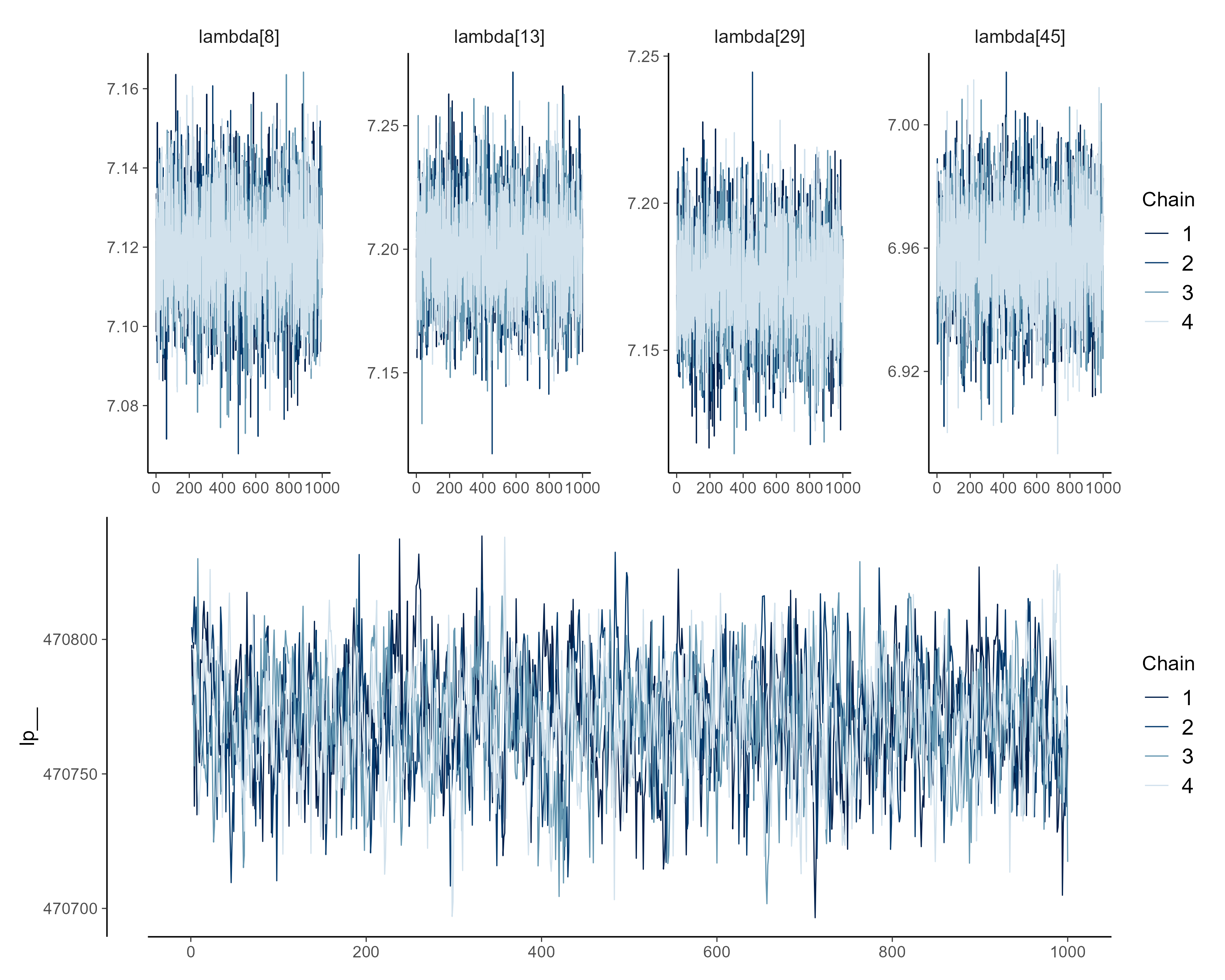

You can also access the underlying cmdstanr fit object for additional diagnostics:

hiv_list$fit$summary()
hiv_list$fit$cmdstan_diagnose()

If diagnostics show divergent transitions or maximum treedepth warnings, first try increasing adapt_delta and max_treedepth. If chains still mix poorly, increase the warmup or sampling iterations and refit:

hiv_list <- run_backcalc(
  sim_diags,
  adapt_delta = 0.99,
  max_treedepth = 14,
  iter_warmup = 1000,
  iter_sampling = 1500
)

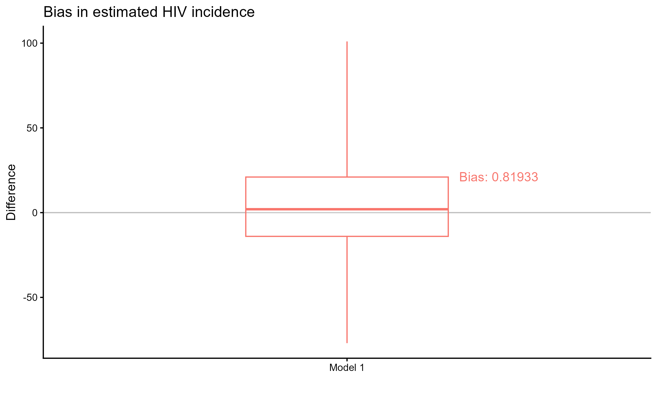
Goodness of fit

When working with simulated data, bias_plot() compares the model estimates against the known simulated values:

bias_plot(hiv_list, quantity = "incidence")

Plot estimates

plot_estimates() produces plots of the posterior estimates with credible intervals. When simulated data is available, the true values are overlaid for comparison.

# HIV incidence over time
p1 <- plot_estimates(hiv_list, quantity = "incidence")

# undiagnosed prevalence over time
p2 <- plot_estimates(hiv_list, quantity = "undiag_prev")

# diagnosis probabilities
p3 <- plot_estimates(hiv_list, quantity = "diag_prob")

# expected diagnoses vs observed
p4 <- plot_estimates(hiv_list, quantity = "diagnoses")

(p1 + p2) / p3 / p4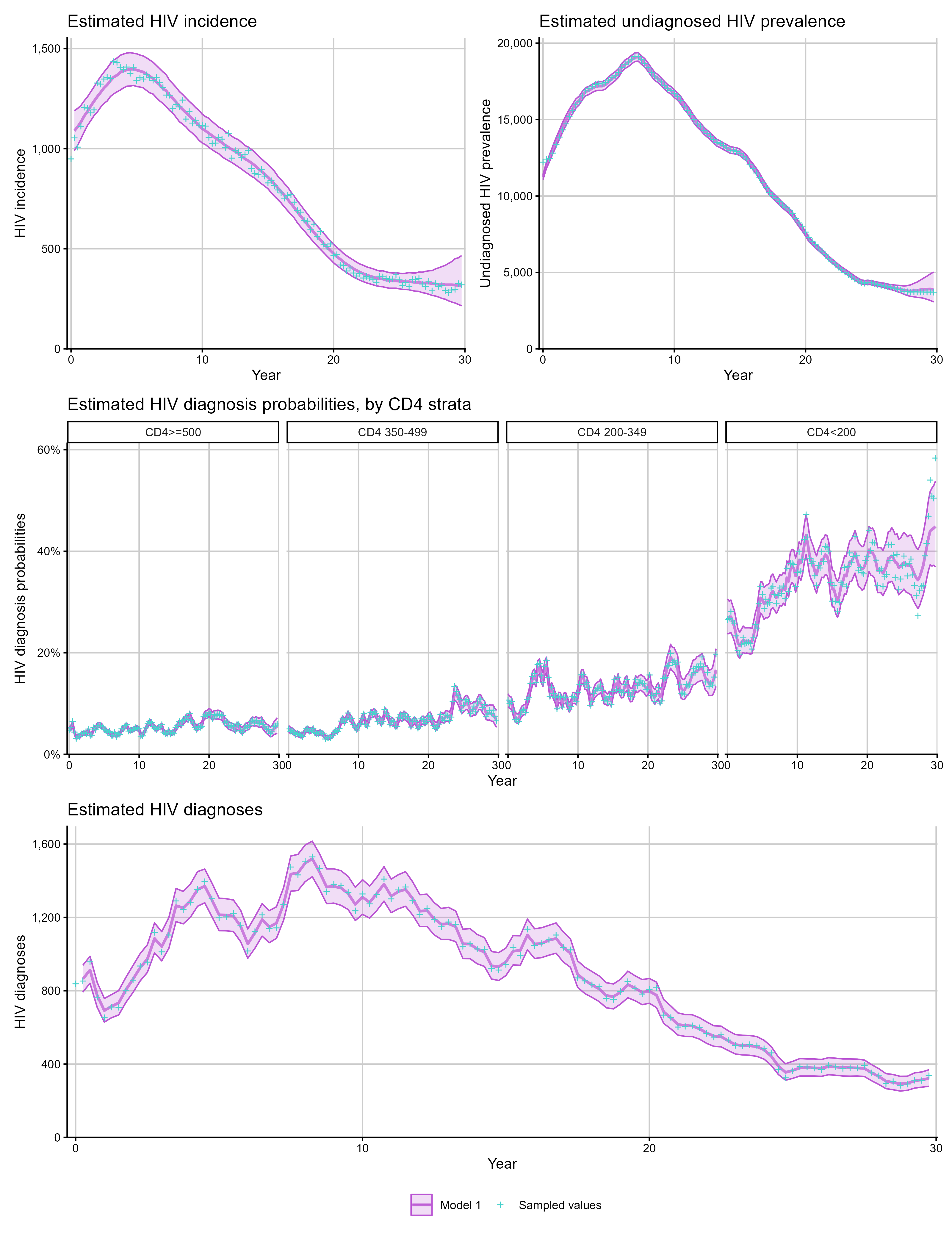

All plotting functions return ggplot2 objects, so they can be further customised:

library(ggplot2)
plot_estimates(hiv_list, quantity = "incidence") +
  theme_gray(14)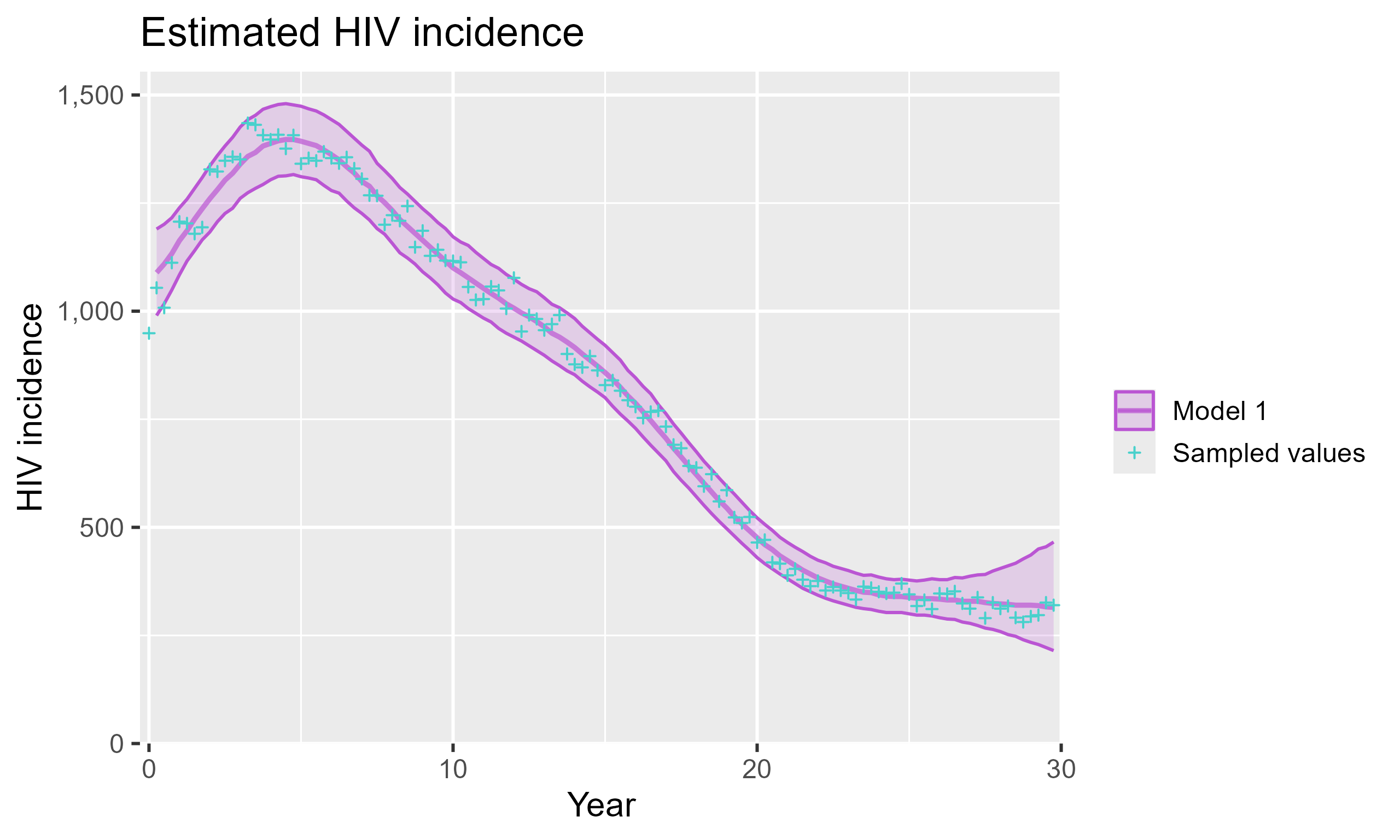

Next steps

• See Model types for fitting models with RITA evidence, migration, and age structure.
• See Analysing results for extracting estimates, comparing models, and the full set of available quantities.
• See Checkpointing for fitting large models in stages on resource-constrained systems.