Analysing results • cd4backcalc

This article covers extracting and visualising results from fitted back-calculation models, including the full set of available quantities, model comparison, and working with real data.

library(cd4backcalc)
library(patchwork)

Available quantities

After fitting a model with run_backcalc(), several quantities can be plotted or extracted. The available quantities depend on the model type:

All models:

Quantity	Description
`"incidence"`	Estimated HIV incidence over time
`"undiag_prev"`	Estimated undiagnosed HIV prevalence
`"diagnoses"`	Expected vs observed diagnoses
`"diag_prob"`	Estimated diagnosis probabilities by CD4 stratum

Migration models (additional):

Quantity	Description
`"all_migration"`	Estimated overall migration with HIV
`"undiag_migration"`	Estimated undiagnosed migration
`"diag_prob_mig"`	Estimated diagnosis probabilities for migrants by CD4 stratum
`"migration_prob"`	Estimated migration probabilities
`"ratio_abroad_uk"`	Proportion of infections acquired in the UK
`"transfers"`	Estimated transfers of care
`"detect_prob"`	Estimated detection probabilities

Age-dependent models (additional):

Quantity	Description
`"incidence_age"`	Incidence stratified by age group
`"undiag_prev_age"`	Undiagnosed prevalence by age group
`"diagnoses_age"`	Diagnoses by age group
`"diag_prob_age"`	Diagnosis probabilities by CD4 stratum and age

Age-dependent migration models (additional):

Quantity	Description
`"undiag_migration_age"`	Undiagnosed migration by age group
`"diag_prob_mig_age"`	Migrant diagnosis probabilities by CD4 stratum and age

Plotting simulated data

Before fitting, simulated quantities can be inspected with plot_simulations():

sim_diags <- simulate_diagnoses(sim_type = "combo_3", migration = TRUE)

p1 <- plot_simulations(sim_diags, quantity = "incidence")
p2 <- plot_simulations(sim_diags, quantity = "undiag_prev")
p3 <- plot_simulations(sim_diags, quantity = "all_migration")
p4 <- plot_simulations(sim_diags, quantity = "undiag_migration")
p5 <- plot_simulations(sim_diags, quantity = "diag_prob")

(p1 + p2) / (p3 + p4) / p5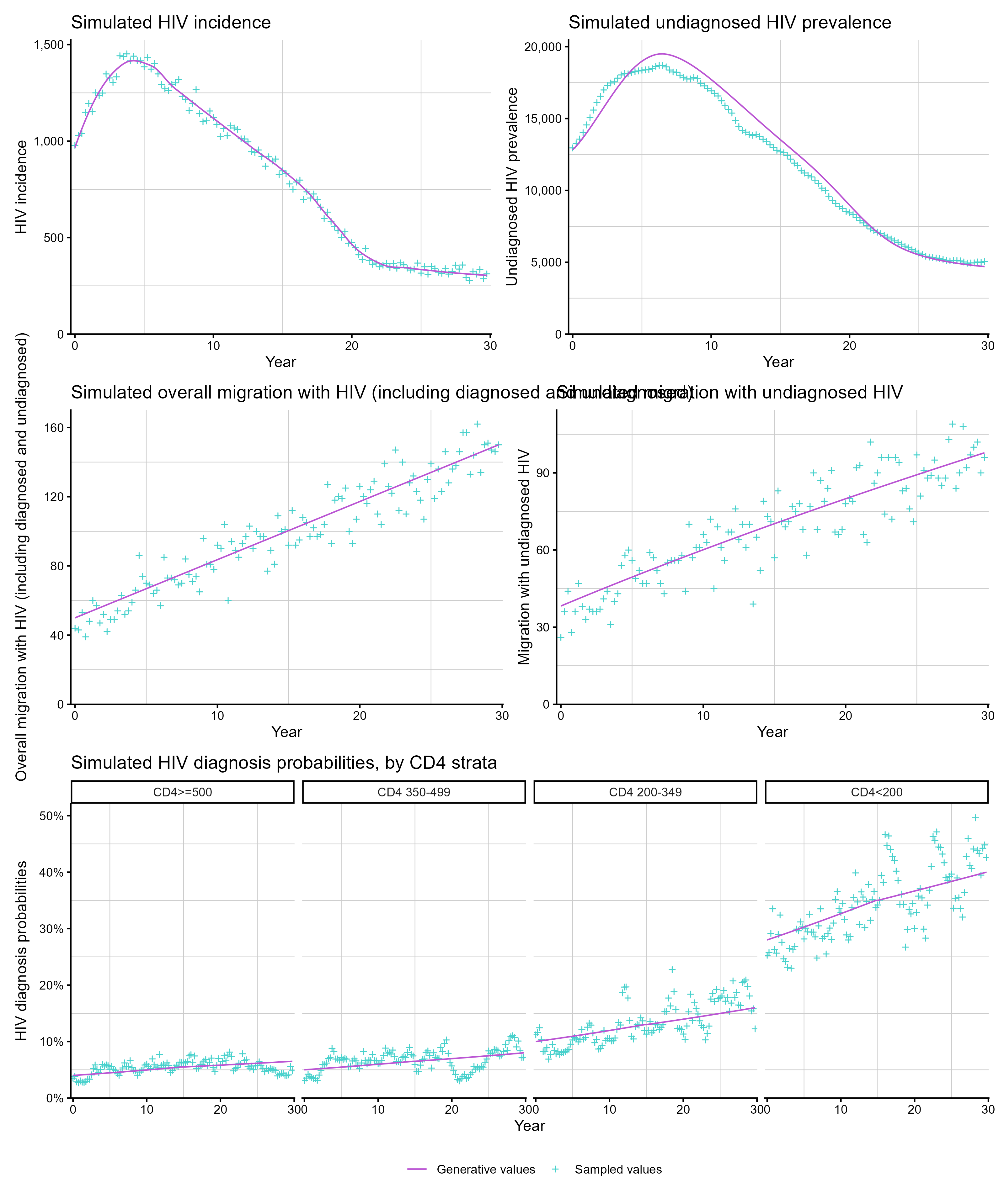

Figure: Patchwork of simulated incidence, undiagnosed prevalence, diagnosis probabilities, all migration, and undiagnosed migration.

Plotting model estimates

plot_estimates() shows posterior median and 95% credible intervals. When simulated data is present, the true values are shown for comparison:

hiv_list <- run_backcalc(sim_diags)

p1 <- plot_estimates(hiv_list, quantity = "incidence")
p2 <- plot_estimates(hiv_list, quantity = "undiag_prev")
p3 <- plot_estimates(hiv_list, quantity = "diag_prob")

(p1 + p2) / p3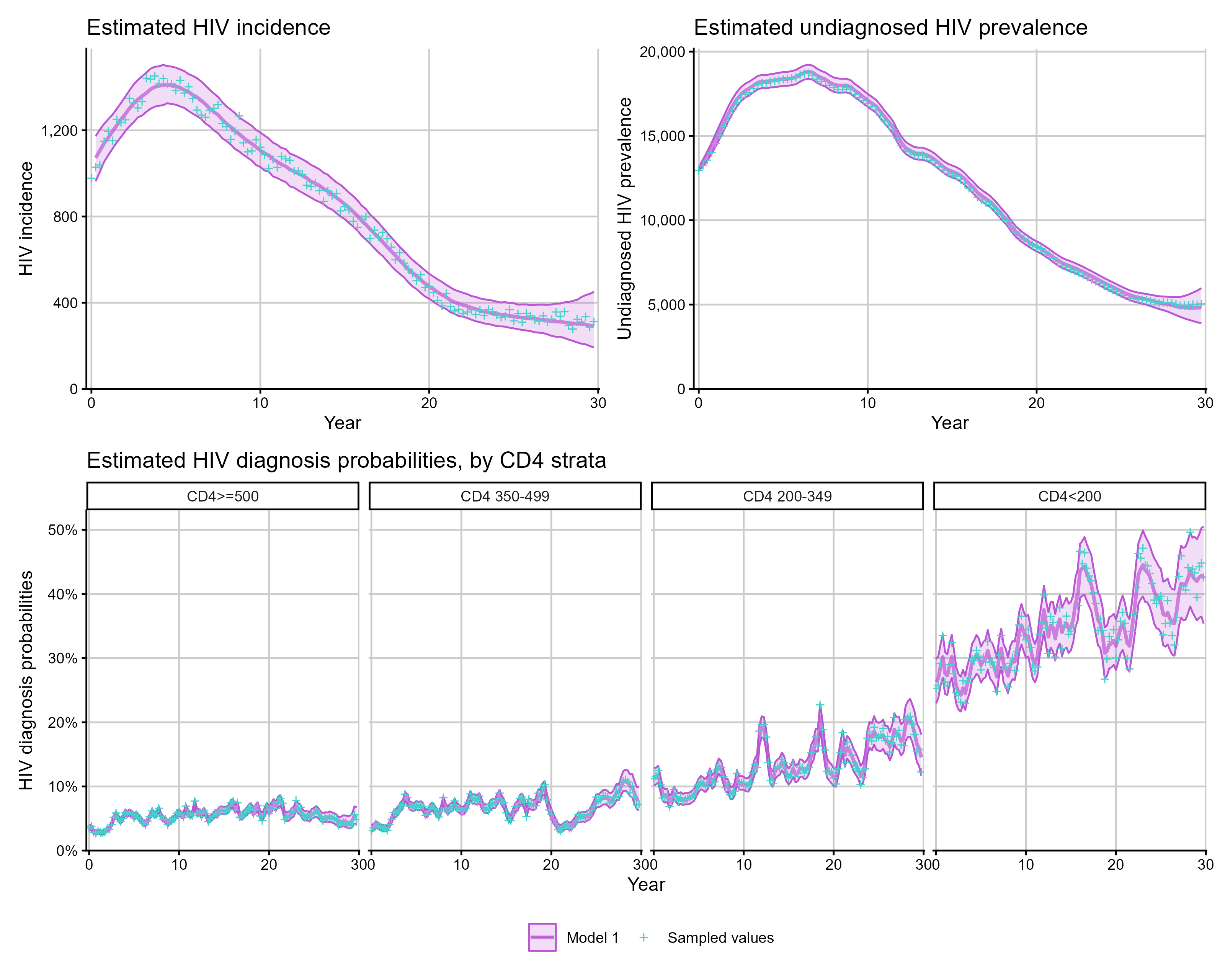

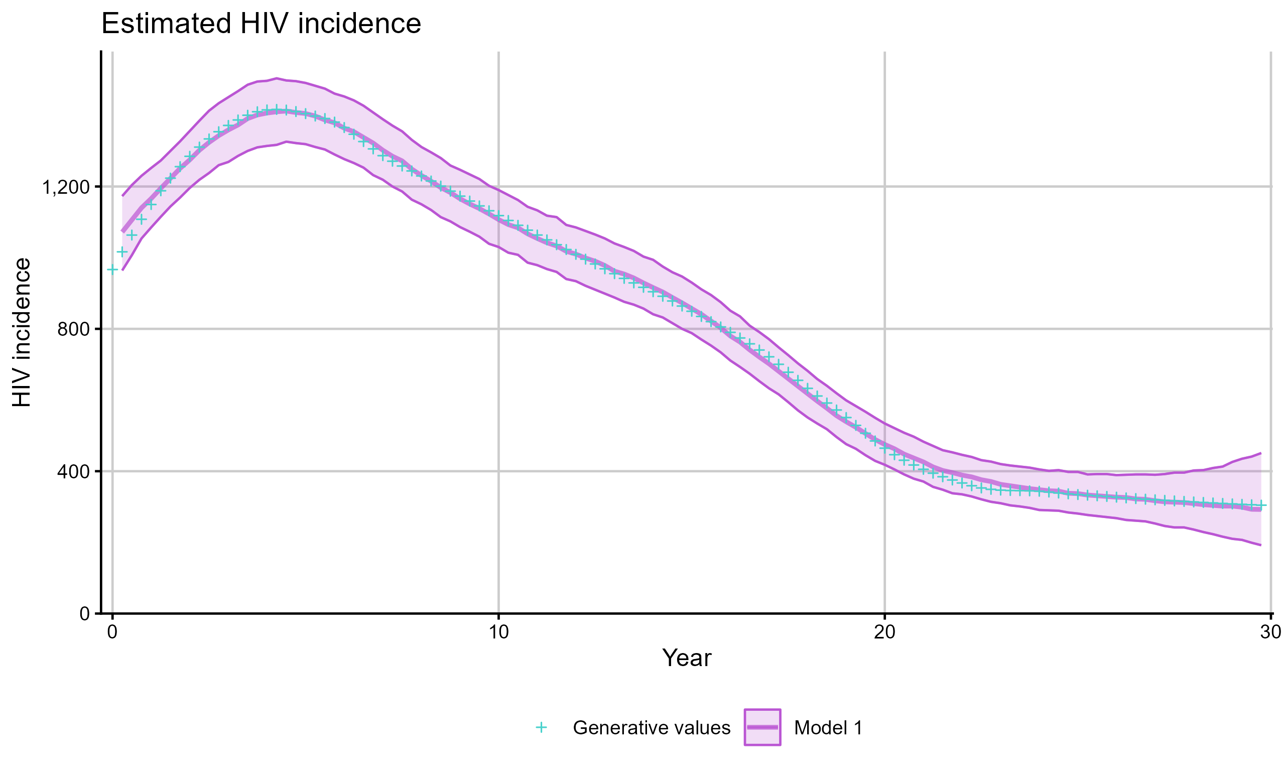
Figure: Patchwork of estimated incidence, undiagnosed prevalence, and diagnosis probabilities.

By default, plotting and summary diagnostics compare fitted values with the sampled realisation from the simulation. To compare against the generative expectation from a particular simulation seed instead, set sim_comparison = "generative":

plot_estimates(
  hiv_list,
  quantity = "incidence",
  sim_comparison = "generative"
)

Figure: Estimated incidence compared against the generative expectation from the simulation.

The same argument is available in bias_plot() and mse_plot().

Extracting estimates as data

Use get_estimates() to obtain the posterior summary as a tibble for custom analysis:

inc_df <- get_estimates(hiv_list, quantity = "incidence")
head(inc_df)

Extracting simulated quantities

Use extract_simulated_quantity() to extract the true simulated values for comparison:

sim_inc <- extract_simulated_quantity(sim_diags, quantity = "incidence")
head(sim_inc)

Use extract_real_data() to extract the observed data used for fitting:

obs <- extract_real_data(hiv_list, quantity = "diagnoses")
head(obs)

Bias and MSE

When fitting to simulated data, bias_plot() shows how much the model over- or under-estimates each quantity and mse_plot() summarises mean squared error across one or more simulated fits:

p1 <- bias_plot(hiv_list, quantity = "incidence")
p2 <- mse_plot(hiv_list, quantity = "incidence")

p1 + p2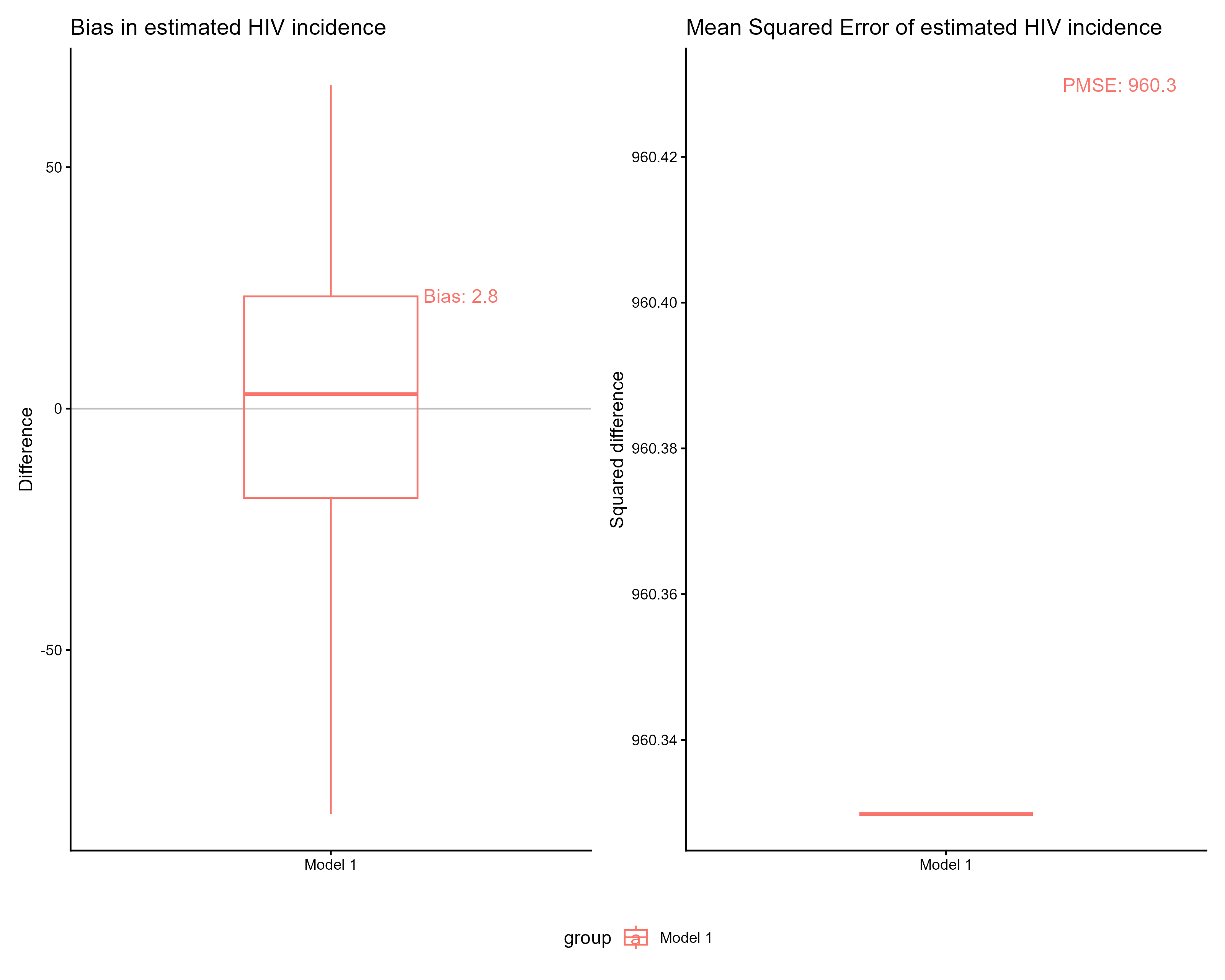

Figure: Bias and MSE plots for incidence.

Comparing two models

plot_estimates(), bias_plot(), and mse_plot() all accept a second model for side-by-side comparison:

sim_diags <- simulate_diagnoses(sim_type = "combo_3", rita = TRUE)
model_rita <- run_backcalc(sim_diags)

sim_cd4 <- sim_remodel(sim_diags, rita = FALSE)
model_cd4 <- run_backcalc(sim_cd4, rita = FALSE)

p1 <- plot_estimates(
  model_rita,
  hiv_list_2 = model_cd4,
  quantity = "incidence",
  model_1_name = "CD4 + RITA",
  model_2_name = "CD4 only"
)

p2 <- bias_plot(
  model_rita,
  hiv_list_2 = model_cd4,
  quantity = "incidence",
  model_1_name = "CD4 + RITA",
  model_2_name = "CD4 only"
)

p1 / p2

Figure: Patchwork of incidence and bias comparisons for two models.

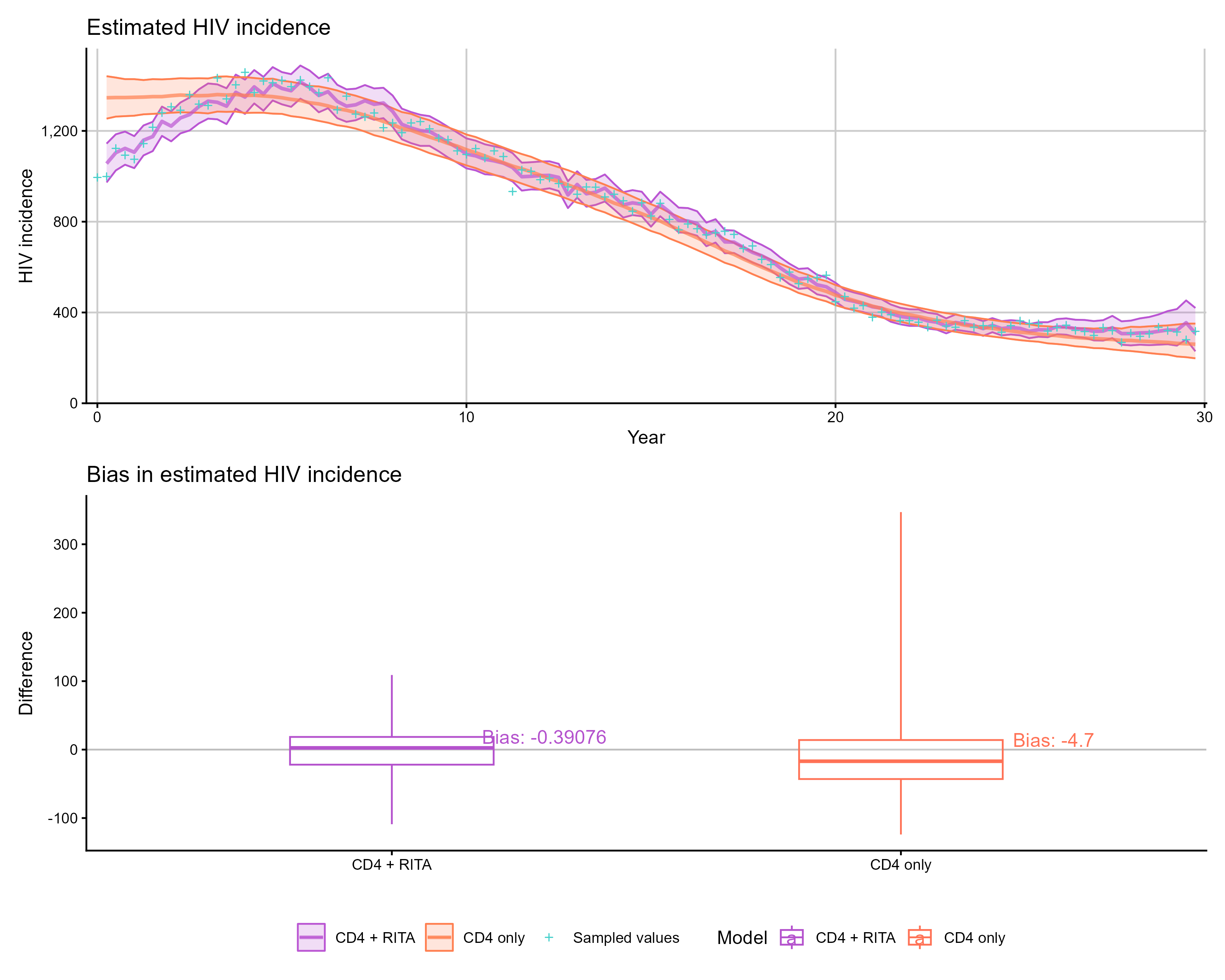
Comparing multiple models

Pass a list of model fits to compare more than two models simultaneously:

sim_diags <- simulate_diagnoses(sim_type = "combo_3")
models <- list()
for (i in 1:3) {
  models[[i]] <- run_backcalc(sim_diags, model_seed = 100 + i)
}

p1 <- plot_estimates(models, quantity = "incidence")
p2 <- bias_plot(models, quantity = "incidence")

p1 / p2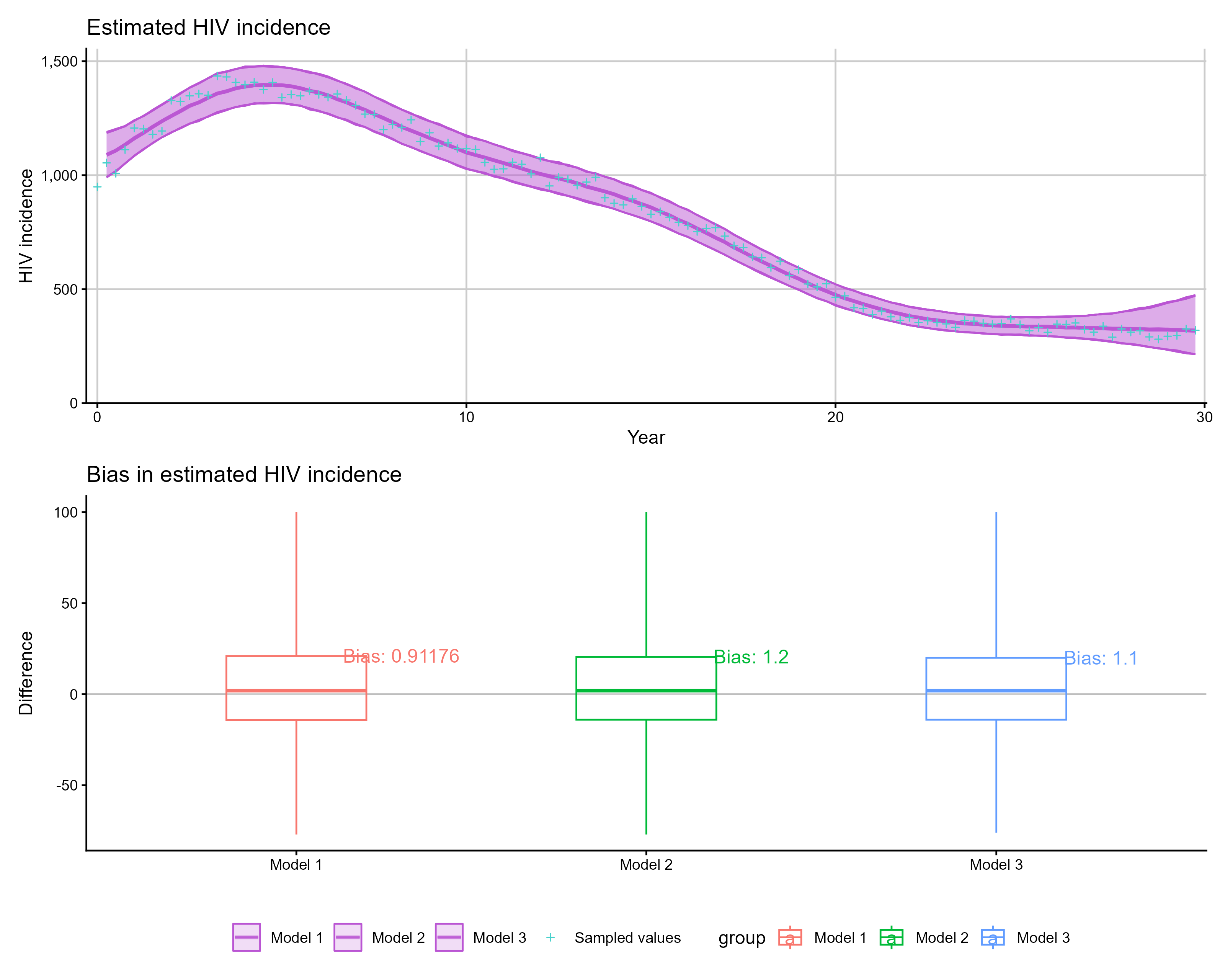

Figure: Patchwork of incidence and bias comparisons for multiple models.

Working with real data

When fitting to real (non-simulated) data, plotting and extraction functions still work — the simulated truth overlay is simply omitted. The stan_data object should contain the diagnosis arrays required for the chosen model, with matching migration, rita, and age flags supplied to run_backcalc().

hiv_list <- run_backcalc(
  real_stan_data,
  migration = TRUE,
  rita = TRUE,
  age = FALSE
)

plot_estimates(hiv_list, quantity = "incidence")
plot_estimates(hiv_list, quantity = "diagnoses")
extract_real_data(hiv_list, quantity = "diagnoses")

Per-chain results

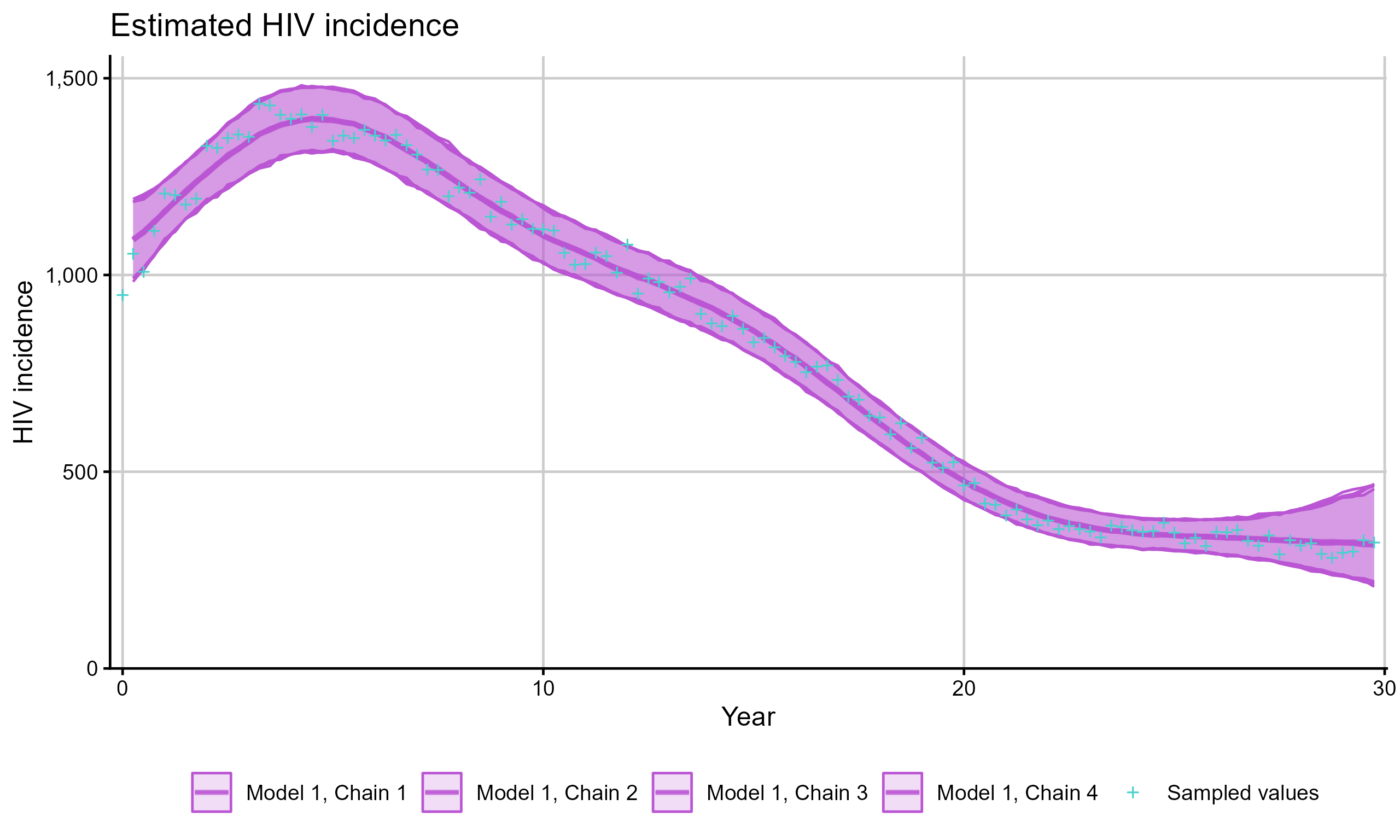
For detailed convergence analysis, set chain_results = TRUE in run_backcalc() to obtain separate posterior summaries for each chain:

hiv_list <- run_backcalc(sim_diags, chain_results = TRUE)
plot_estimates(hiv_list, quantity = "incidence", chain_results = TRUE)

Figure: Per-chain incidence estimates.